Grandpa troll

This is a model I made from a little grandpa troll statue. First I took digital pictures of the statue from strategic view: front, left and top. Then scale the pictures so the model has the same size from the different views. All the views were merge into a following single picture which I used as reference for the modeling. And here is the topology of the head.

Skeletal animation, Blender and math... continue

In a preview post, I have written about my 3d engine and skeleton animation. My goal was to export an animation from Blender (2.49) and play it back into an another program. This is achieved now and works correctly.

But I have met problems because I misunderstood the different coordinate spaces involved and how they are related to each other in Blender. When you understand those coordinate spaces, a big part of the game consist of using the good maths to build back the animation.

Let's explore the blender skeletal animation system with a special focus on the different coordinate spaces. When you know/understand the needed informations, you can export them by using the Blender Python API.

Armature

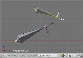
An armature is a hierarchal set of bones. One bone can have several children. One bone has none or one parent. The picture below shows two bones. The top one and the bottom one are respectively the child and the parent . This is indicated by the dashed line. A bone can be connected or not to its parent. Connected means that the child's head is at the same position of the parent's tail, and it will remains as this while editing. This feature is useful while editing the armature for structure as arms or spine. But as we are not interested in editing but playing back the animation, this information is not important.

Bone anatomy

The picture below shows one bone in edit mode. A bone is composed of two points, the head and the tail, represented by the spheres, respectively at the bottom and the top of the bone. There are other parameters that characterize a bone, but I would like to focus on those.

In Blender, when you had an armature into a 3d scene (Shift A, Add > Armature), you obtain one bone of one unit length pointing in the world z-axis, as in the picture above. So far, problems arise, and it is about he bone axis... thus the bone space.

The bone space

When you enable bone axis drawing in the Armature tab from the editing panel (F9), you notice that the bone axis (in white) are not align with the world axis (red, blue, and green). And that is very disturbing at first sight because of this counter-intuitive aspect.

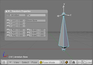
The picture above shows the same bone but in pose mode. By looking the transform properties floating panel you notice that the bone has not been rotated (RotX/Y/Z is 0). Hmmm, so, why the bone axis are not aligned with the world axis? Because bone are really typical object in Blender. They are different from other objects such as mesh, camera, or light, about how local axis is defined.

When you edit an armature, you are basically defining bones hierarchy and placing points as bone heads and bone tails. As a bone is defined by two points, you can not tell how a bone is rotated. Until a convention is defined.

The convention used in blender is as followed:

• The Y axis is aligned along the bone length, that is the normalized vector formed by the head and tail points.
• The X and Z axis has the same coordinates as Y, but rotated. That is X=(Yy, Yz, Yx), Z=(Yz, Yx, Yy).
• A rotation angle around the Y axis is defined. Called "Roll" in the properties panel in edit mode.

X, Y, Z formed the bone space. Which is important for the animation because as you will see in the next chapter, the transformations are expressed in that space.

For this purpose, the essential information about the structure of the armature are, for each bone:

• its name
• the name of its parent (if it has one)
• its transform matrix in armature space
• its rotation matrix in bone space

Animation curves

The picture below is a screen-shot of the Ipo Curve Editor displaying pose curves of one bone. This is visible by selecting "Pose" from the "Ipo Type" combo-box. Here again, you can see that bones are very specific.

Compared with Object Ipo Curves, Bone Ipo Curves are very basic. The ten curves concern "only" the three transformations: translation (LocX, LocY, LocZ), rotation (QuatW, QuatX, QuatY, QuatZ), and scaling (ScaleX, ScaleY, ScaleZ). Notice that quarternion are used for rotation, that's why the x,y,z values vary between 0 and 1, and w between -1 and 1.

One important point to note down for later : those transformations are expressed in bone space.

The skin

The aim of skeletal animation is to deform a skin by moving bones. The skin is often a mesh which is a bunch of connected vertices forming edges and faces. When a bone moves, it also moves the vertices associated to it, thus the skin.

In Blender, bones and vertex groups are associated when they have the same name.

The picture above illustrates the association of a skin and a skeleton. On the left the Outliner Window shows two Vertex Groups named "bottom" and "top", the latter is selected. One the right the 3D Window, in Weight Paint mode, shows the Vertex Groups "bottom" and "top" respectively in blue and red. The armature with the bone names are displayed.

The vertex coordinates of the mesh are expressed in the object space.

The animation: the all together

We have seen all the elements involved in skeletal animation. Let's resume all the informations we can retrieve by the Blender Python API.

• The skin: the vertex coordinates in object space
• The skeleton: the bones hierarchy and transform matrices in armature space and in bone space
• The bone animation curves in bone space
• The vertexgroups

The skin and the skeleton is either in bind pose or current pose (see this presentation for explanation of those poses). The armature and the mesh are exported in bind pose. The goal is to compute the vertex positions of the mesh in current pose.

Let v the position of a vertex in bind pose in object space and v' its position in current pose. We know v and we have to compute v'.

As the animation curves are expressed in bone space, we need the vertex position from object space v in that space. This is done by multiplying the vertex position in object space v by the inverse of transform matrix in armature space B of the bone b associated with the vertex.

v_bonespace = inv(B_b)v

Then, we multiply this by the transform matrix P_b computed from the animation curves of the bone b. We obtain v' in bone space.

v'_bonespace = P_bv_bonespace

What is left now, is to compute back that position in the armature space. For this we multiply it by the matrix product of rotation and translation of each bone in current pose, from the bone of interest to the root bone. That's it =).

Skeletal animation, Blender and math

I am implementing a basic graphic engine. So far the engine can, briefly, load textured 3d models from an OBJ files and render them. I am making this engine with the idea of making an abstraction layer over OpenGL in order to manipulate 3d objects as simply as possible...

Now, I am adding skeletal animation to the engine. I have created a python script to export an armature and its animation from Blender into a home-made-OBJ-like-formated file (OBJ does not support animation). The engine can load that file, so an armature can be attached to a mesh in order to deform the latter. I broke my teeth implementing the skeletal animation and get lost into the maths. As a result, I obtained distorted animation, far from satisfying.

Thus, I decided wisely to learn about the math around skeleton animation. After some searches, I have found a very interesting presentation from a video game programming course in which all the maths I need were in, described concisely. I suggest to read this presentation to anyone who want to know about skeletal animation from a mathematical point of view. It is really crystal clear, as I like. Thanks to Jason Gregory.

Island

One animation I have made for fun using the 3d software suite Blender. The music is from the Impossible Mission original TV series.

The crab is animated as one block, without armature. By looking at it you will noticed that any part of its body does not move independently.

The water splashes are made by using the Blender particles system. It looks more as smoke than as water. I should take more time on that if I had to do it again.

My 1st full model in Google Earth

This is my first full architectural 3d model published in the Google Earth Buildings layer. Full because this one is fully textured in contrast with my last model (read this post if you want to know more).

Town hall 3D model story

Ten months ago, I have created this architectural 3d model of the old town hall of my city of birth. I have uploaded it on Google 3D Warehouse and made a request to publish it on the 3D buildings layer of Google Earth. My model was on the review queue waiting to be accepted.

Five months later, I received a review message: improvements needed before acceptation. The improvements to be done was not so explicit. Indeed I get an indication on which criteria my model did not fit. It was "Incomplete Texture". And it was sadly true...

That was not an error or missing, nothing else but my willing. The problem here was that I had no pictures of this part of the building. And instead of create something that does not exist in reality, I preferred to leave this part as it is (with this fancy plain color).

Correcting this is not a huge task. I could have textured it with some default wall texture and submit the model again. This could have solve the problem, Google reviewers would have been happy with it and it would still indicated an absence of information. But I was busy during that time and just forgot about it. Another pertinent excuse is: there is no Linux version of Google SketchUp (I am using mainly Linux now).

Recently, I was surprised to see a blue ribbon next to my model, indicating that it has been published on the Google Earth 3D buildings layer. I wondered how that could be since I have made any "improvements", it should have not been published. I was curious to see if that was true. I had a look on Google Earth and it was effectively there...

... at least partially.

Apparently the motto is : "Fully textured or not textured at all!"

What a binary world...

Trackball view rotation

Introduction

Often we would like to visualize a 3d model from different view angles. Trackball is rotation technique that allow the user to intuitively change the view angle by using the mouse. The mouse behaves like a virtual trackball. Let's try to understand how trackball view rotation work exactly. This could be useful, as a programmer, if you want to implement this rotation technique in your application. Or if your are an artist it could be interesting to know what's happen under the stage.

Principle

The mouse moves on the screen which is a 2D plane. However a trackball could rotate in any direction in a 3D space. The problem here is to match the planar mouse movement to a 3D rotation. The idea to solve this problem is to project the 2D coordinate of the mouse cursor on a virtual sphere behind the screen, thus we obtained 3D point (blue on the picture). The difference between this 3D point and the center of the virtual sphere (red on the picture) is a 3D vector. The movement of this 3D vector while dragging the mouse is a rotation around the sphere center. Here we are! We use that rotation to rotate the view.

Transformation matrices

"Unfortunately, no one can be told what the Matrix is. You have to see it for yourself." Morpheus, The Matrix - 1999

Introduction

Matrices in 3D applications are very useful tools. Translation, scaling and rotation in any combination are simplified by usage of matrices. Let's expose the most important statements:

1. Any transformation in space can be describe by a matrix
2. Transforming a point in space is done by multiplying a transform matrix by the column vector describing the coordinates of the point
3. Several successive transformations can be resumed as one matrix

The maths

So if you want to perform a transformation on a point, all you have to do is to select the appropriate matrix (see below) plug in the parameter values (position, scaling factor, angle, or rotation axis) and multiply it with the column vector of the point coordinate.

Let's detail this, mathematically. The transformation can be written as:

v' = Mv

Where:
v a column vector describing the coordinate of the point (x, y, z, w) w = 1 most of the time
M a 4-by-4 matrix describing the transformation
v' a column vector describing the coordinate of the point after the transformation (x', y', z', w')

According the definition of matrix multiplication, we obtain

x'       a  b  c  d   x      ax + by + cz + dw
y'       e  f  g  h   y      ex + fy + gz + hw
z'   =   i  j  k  l . z   =  ix + jy + kz + lw
w'       m  n  o  p   w      mx + ny + oz + pw

Now, about the statement 3, it is again related to matrix multiplication. The result of 4-by-4 matrices multiplication is also a 4-by-4 matrix and it still a transformation.

And matrix multiplication is not commutative (AB is not BA). That is a good for us, it means that we can also describe the order of the transformations. Let's say we have point v and we would to transform it by a rotation R followed by a translation T.

v' = RTv

One remark here, we noticed that if we read from left to right, the rotation appear first. But that doesn't means that the rotation is perform first. The order of transformation is readed from right to left.

Another magical thing, suppose we have a complete 3D object. Transforming a 3D object is transforming all of its points. Instead of performing the rotation, follow by the translation to each point. We compute, once for all, the matrix that describe the combination of these two transformations, let's call it M. And then, multiply M by each point.

M = RT
for each point: v' = Mv

It does not matter how many transformations is performing, M will always describe them all. Magic! isn't it ?

Here is a list of of basic transformation matrices: translation, scaling, and rotation.

Translation matrix

X, Y, Z are the components of the translation vector.

1  0  0  X
0  1  0  Y
0  0  1  Z
0  0  0  1

Scaling matrix

X, Y, Z are scales factors along their respective axis.

X  0  0  0
0  Y  0  0
0  0  Z  0
0  0  0  1

Rotation around the x axis by an angle a

1   0   0   0
0   c  -s   0
0   s   c   0
0   0   0   1

Where c = cos(a) and s = sin(a)

Rotation around the y axis by an angle a

 c   0   s   0
 0   1   0   0
-s   0   c   0
 0   0   0   1

Where c = cos(a) and s = sin(a)

Rotation around the z axis by an angle a

c  -s   0   0
s   c   0   0
0   0   1   0
0   0   0   1

Where c = cos(a) and s = sin(a)

Rotation around an arbitrary axis by an angle a

x, y, z are the components of a unit vector that represent the rotation axis.

t*x*x + c        t*x*y - z*s     t*x*z + y*s     0
t*x*y + z*s      t*y*y + c       t*y*z - x*s     0
t*x*z - y*s      t*y*z + x*s     t*z*z + c       0
0                0               0               1

Where: c = cos(a), s = sin(a), and t = 1 - c